PG-Strom SSB Benchmark — Arrow FDW Comes Before GPU

Reading the PG-Strom documentation for the first time, the pitch sounds clean: install an extension, and queries run on the GPU. Across 555 test cases on three server environments, the reality is more specific. Without Arrow FDW, you get 1.6× acceleration. On wide tables, GPU+Heap is slower than CPU alone. With Arrow FDW, you get 10× at 600GB scale. The difference is not GPU specs. It is how much data has to reach the GPU and how fast.

---

What PG-Strom Does and Where the Bottleneck Is

A standard PostgreSQL query follows this path:

Disk (SSD/NVMe) → OS page cache → shared_buffers → CPU executor → result

With PG-Strom active, aggregation, scan, and filter operations are offloaded to the GPU:

Disk → OS page cache → RAM → PCIe bus → GPU VRAM → CUDA kernels → result

A GPU like the L40S has 18,176 CUDA cores executing the same operation in parallel. SUM(price * discount), GROUP BY region — these map directly onto that parallel architecture. A CPU handles the same computation with tens of physical cores.

But those 18,176 cores sit idle until data arrives in VRAM. The PCIe bus connecting CPU and GPU is the transfer channel.

PCIe 4.0 ×16 theoretical bandwidth: ~32 GB/s

Reading from disk means traversing: NVMe → CPU RAM → PCIe → GPU VRAM. Every byte of data travels that path before a single CUDA kernel can touch it. GPUDirect Storage (GDS) short-circuits CPU RAM out of the path (NVMe → PCIe → GPU VRAM), but Server B's GDS was disabled to measure baseline NVMe I/O behavior independently.

PCIe transfer cost is the actual performance determinant. GPU core count and CUDA version matter less than how much data gets sent.

---

Three Test Environments

Server	CPU	GPU	Storage	Purpose
Server A	Xeon Gold 6526Y ×2 (32C/64T, 2.8–3.8GHz)	L40S 48GB ×3 (single GPU active, license limit)	SATA SSD 1.92TB ×4	Basic SSB + GPU Cache
Server B	Xeon Gold 6448H ×2 (64C/128T, 2.4–4.1GHz)	L40S 48GB ×1 (PCIe 5.0)	NVMe SSD 894GB ×2	Scale Factor 1→100 sweep
Server C	GCP g2-standard-4 (2C, 16GB RAM)	L4 23GB ×1 (PCIe 4.0)	NVMe 375GB + 100GB	OLAP engine comparison + vector search

The L40S is an Ada Lovelace GPU: 48GB VRAM, CUDA 13.0. The L4 is an entry-class cloud GPU. Server A has three L40S cards but only one is active due to XCruzDB licensing.

The benchmark workload is Star Schema Benchmark (SSB) queries q1.1–q4.3, 13 queries total. SSB is a data warehouse benchmark derived from TPC-H, centered on JOIN aggregations between a large lineorder fact table and small dimension tables (supplier, customer, part, date). Scale Factor 1 = ~6M rows / ~6GB; SF=100 = ~600M rows / ~600GB.

Every query was measured in both cold cache (OS cache dropped) and warm cache states. Each query ran at least 5 times; the target coefficient of variation was below 10%.

---

Heap vs Arrow FDW — The Storage Format Decides Everything

Understanding Arrow FDW is the prerequisite for understanding PG-Strom.

PostgreSQL Heap Storage

PostgreSQL's default storage is Heap: row-oriented. A table with 17 columns stores all 17 column values consecutively per row.

Page 1:
  [row1: lo_orderkey, lo_linenumber, lo_custkey, ..., lo_supplycost, lo_revenue]
  [row2: lo_orderkey, lo_linenumber, lo_custkey, ..., lo_supplycost, lo_revenue]
  ...

SSB q1.1 touches four columns:

SELECT SUM(lo_extendedprice * lo_discount) AS revenue
FROM lineorder, date
WHERE lo_orderdate = d_datekey
  AND d_year = 1993
  AND lo_discount BETWEEN 1 AND 3
  AND lo_quantity < 25;

lo_extendedprice, lo_discount, lo_orderdate, lo_quantity — four of seventeen. Heap storage reads the entire row regardless. All 17 columns go from disk to RAM to PCIe to GPU VRAM, even though 13 will be discarded immediately.

Apache Arrow FDW

Arrow FDW reads Apache Arrow columnar format files as a PostgreSQL Foreign Data Wrapper. Arrow stores data column-by-column in contiguous memory blocks:

Arrow file layout:
  [lo_orderkey block:      v1, v2, ..., v6M]
  [lo_linenumber block:    v1, v2, ..., v6M]
  ...
  [lo_extendedprice block: v1, v2, ..., v6M]
  [lo_discount block:      v1, v2, ..., v6M]
  ...

For q1.1, Arrow FDW reads only the four needed column blocks. 4 of 17 columns — roughly 24% of the I/O that Heap requires.

The PCIe Math

lineorder at SF=1 (~6M rows):

• Heap: 17 columns × 8 bytes avg × 6M rows ≈ 816MB to transfer
• Arrow FDW (4 columns): 4 × 8 × 6M ≈ 192MB

PCIe 4.0 ×16 transfer time:

• Heap: 816MB ÷ 32GB/s ≈ 25ms (theoretical)
• Arrow: 192MB ÷ 32GB/s ≈ 6ms

In practice, disk I/O and DMA overhead add to both, but the ratio holds. Arrow FDW sends less data, so GPU cores get to work sooner.

---

SF=1 Results — Same GPU, Same Queries, Different Storage

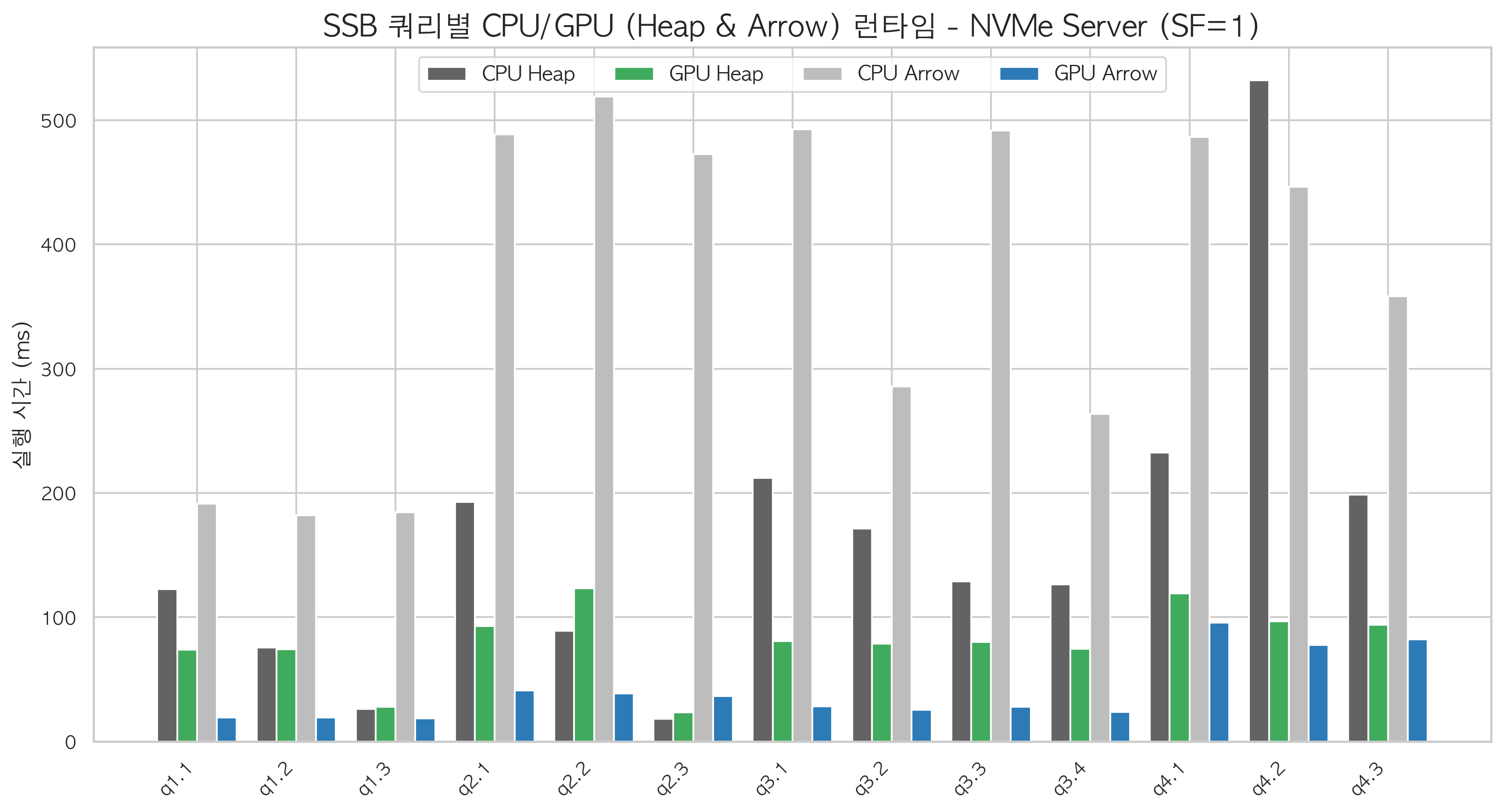
Server B (NVMe, L40S), 13 SSB queries at SF=1.

Combination	GPU/CPU speedup
Arrow + GPU	12.4×
Arrow + CPU	baseline
Heap + GPU	1.6×
Heap + CPU	baseline

Same L40S. Same queries. Arrow gives 12.4×; Heap gives 1.6×.

The extreme case: on wide tables with 50+ columns when only 2–3 columns are selected, Heap+GPU was 18–27% slower than CPU alone.

The numbers explain it. A 50-column table with 8 bytes per column averages 400 bytes per row. Reading 10M rows from Heap: 4GB must transfer across PCIe. At 32 GB/s: 125ms of transfer time. During those 125ms, every GPU core waits. The actual aggregation — SUM, GROUP BY — takes a few milliseconds. Transfer latency overwhelms computation benefit.

CPU has no such penalty. Data already in shared_buffers or OS page cache is processed through L3 cache almost immediately. So for Heap on wide tables: "cost of sending data to GPU > benefit of GPU computation."

Arrow FDW sends only 2–3 column blocks. Transfer time drops to 4–6ms. GPU cores start working immediately.

The PG-Strom performance formula is not about GPU core count. It is minimize transfer × parallelize computation. Arrow FDW handles the first half; GPU handles the second.

---

Scale Factor 1→100 — Larger Data, Larger Gap

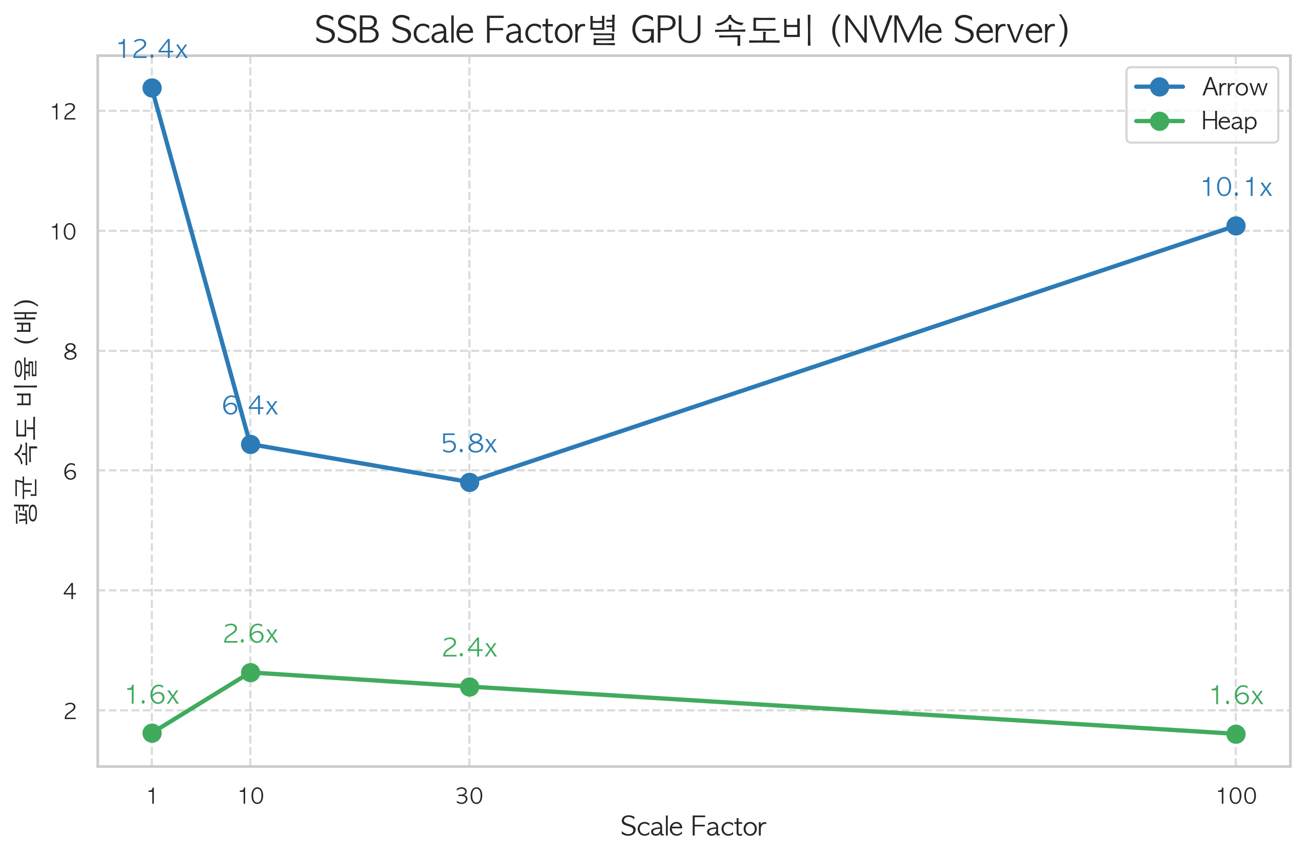
Server B (NVMe), full SF sweep.

SF	Data size	Arrow GPU/CPU	Heap GPU/CPU	Arrow+GPU total	CPU+Arrow total
1	~6GB	12.4×	1.6×	4.6s	36.5s
10	~60GB	6.4×	2.6×	5.9s	28.3s
30	~180GB	5.8×	2.4×	14.1s	65.2s
100	~600GB	10.1×	1.6×	21.5s	221.0s

The SF=30 dip happens because NVMe sequential read bandwidth approaches saturation. Even with column-selective reads, absolute I/O volume grows with data size, and both CPU and GPU end up waiting on storage.

At SF=100, the speedup recovers to 10×. Queries at this scale reference fewer columns relative to total table width, so Arrow FDW's column-selection benefit is maximized. In absolute time: 21.5 seconds versus 221 seconds for the same 13 queries. Ten times faster.

Heap+GPU flatlines at 1.6× regardless of SF. As data grows, PCIe transfer time grows proportionally, continuously diluting whatever acceleration the GPU provides.

---

GPU Cache — Eliminating the PCIe Bottleneck Entirely

Arrow FDW still incurs PCIe transfer on every query. Installing a gpucache trigger on a table keeps the data resident in GPU VRAM permanently. Subsequent queries have zero disk or PCIe cost.

Server A, t_big_cache (10M row aggregate):

Case	GPU ON	GPU OFF	Speedup
t_big_cache (GPU Cache active)	39.26ms	2,525.79ms	64.3×
Arrow FDW full scan (346MB)	21.34ms	810.58ms	38.0×

GPU Cache is 1.7× faster than Arrow FDW because there is literally nothing to transfer. GPU cores operate directly on VRAM-resident data.

Operational constraints narrow the applicability:

Good candidates:

• Tables smaller than VRAM (L40S: 48GB)
• Infrequently updated, frequently aggregated tables — dimension tables (dates, regions, product codes), lookup references

Poor candidates:

• Multi-hundred-GB fact tables — exceed VRAM
• High-frequency write tables — the gpucache trigger must sync VRAM on every INSERT/UPDATE/DELETE

A practical mixed strategy: GPU Cache for dimension tables, Arrow FDW for large facts.

---

Comparison With Other OLAP Engines

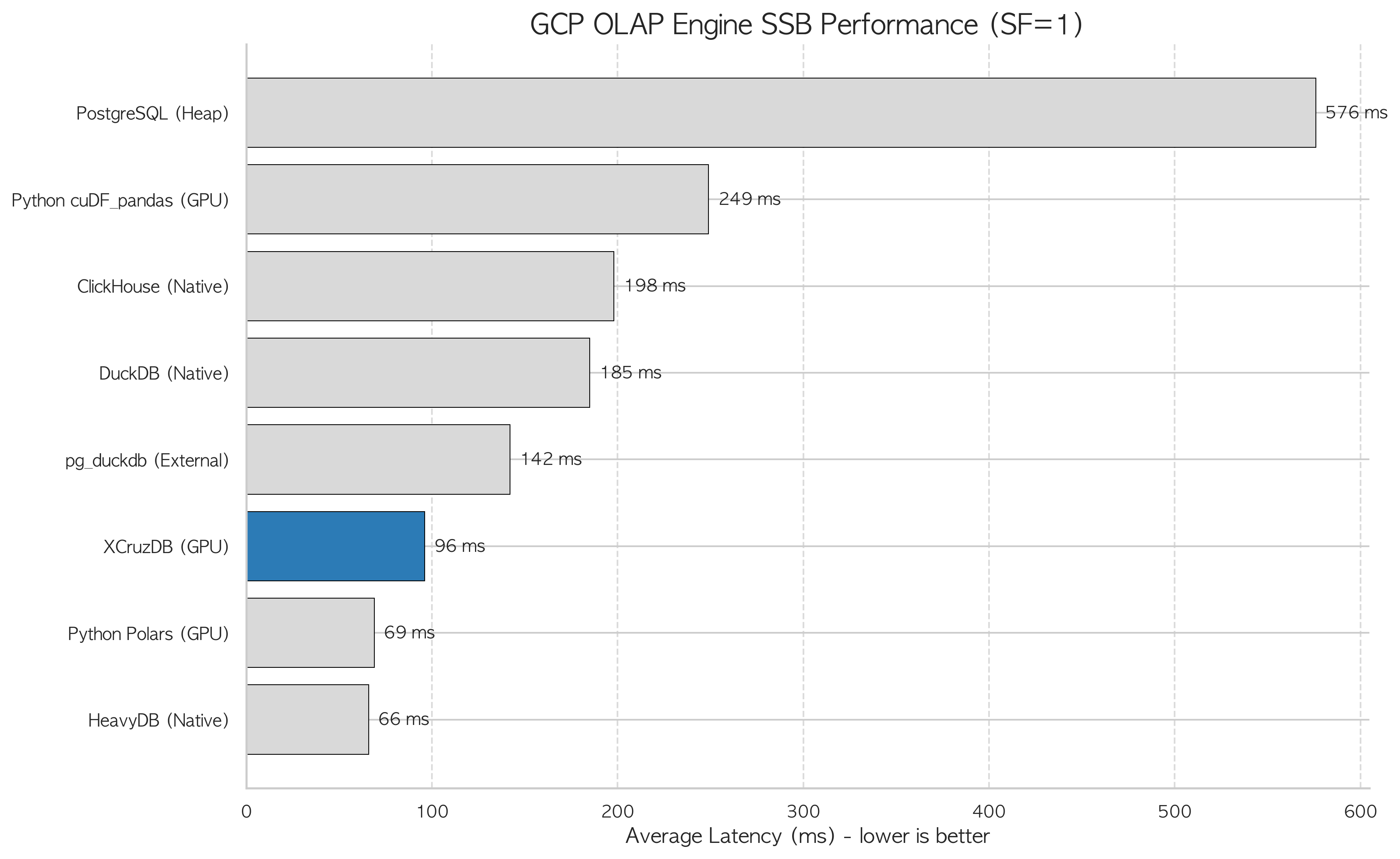
GCP Server C (L4 GPU), SSB SF=1, 13-query average.

Rank	Engine	Avg runtime (ms)	vs PG Heap	Notes
1	HeavyDB	66	8.7×	GPU-native DB, warm cache
2	Python Polars (GPU)	69	8.3×	Lazy eval + GPU RAPIDS
3	PG-Strom/XCruzDB (GPU)	96	6.0×	PostgreSQL ecosystem preserved
4	pg_duckdb (Parquet)	142	4.2×	PG+DuckDB hybrid, no GPU needed
5	DuckDB native	185	3.1×	CPU vectorized, separate process
6	ClickHouse	198	2.9×	CPU columnar DB
—	Python cuDF_pandas	249	2.4×	pandas API on GPU
—	PostgreSQL Heap	576	baseline	—

HeavyDB is the fastest at 66ms — a GPU-native database architecture. But it requires migrating away from PostgreSQL entirely: schemas, application queries, pgvector indexes, PostGIS usage, monitoring configurations.

PG-Strom delivers 96ms while staying inside PostgreSQL. It is roughly 2× faster than DuckDB and ClickHouse while keeping the full PostgreSQL stack intact.

pg_duckdb at 142ms (4.2×) is notable: it achieves this without a GPU, by embedding DuckDB inside PostgreSQL to read Parquet files. For teams without GPU hardware, pg_duckdb represents a meaningful OLAP acceleration path through columnar I/O efficiency alone.

---

GCS: The Cloud Storage Reality

Separate from the NVMe measurements, we ran all 22 TPC-H SF=100 queries (~100GB, ~866M rows) against GCS to establish a realistic baseline for object-storage-backed Lakehouse deployments.

Storage environment	Performance vs NVMe
Local NVMe	baseline (1×)
GCS cold query (first execution)	~650× slower
GCS + session cache (re-execution)	~2.6× slower

The first query against GCS runs 650× slower than NVMe. Reading 100GB of objects over HTTP/TLS means network latency, GCS throughput limits, and transfer overhead that NVMe simply does not have.

Session cache brings the second execution down to 2.6× slower than NVMe. This assumes the previous query's data is still cached — a different filter, a different table, or cache eviction restores the cold penalty.

All 22 TPC-H queries completed successfully, and correctness at SF=100 scale is confirmed. But building production query SLAs on GCS without a caching strategy is a risk. "Fast ad-hoc" on cloud object storage means cache-hit ad-hoc.

---

Vector Search: cuVS vs pgvector

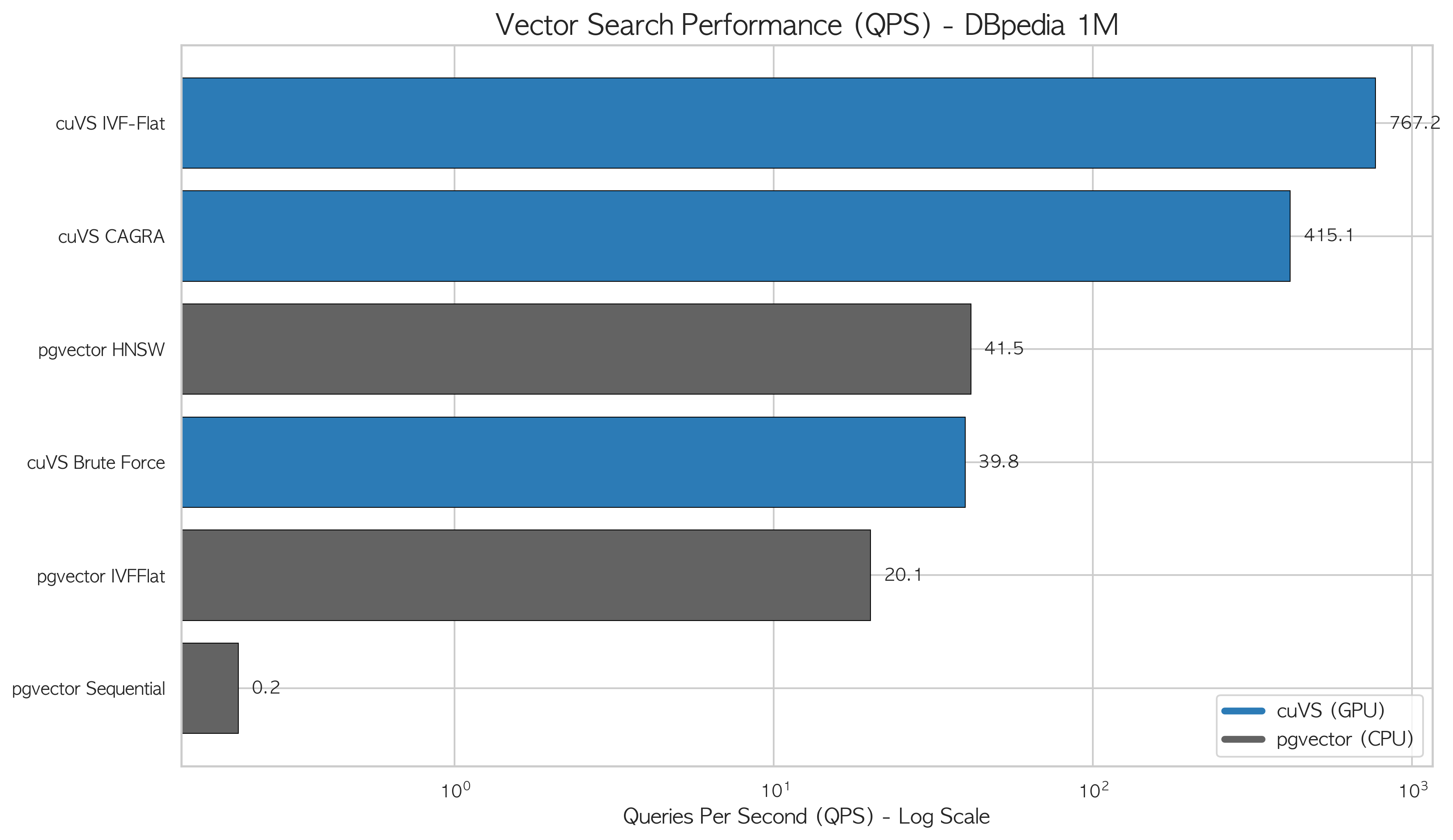
As a secondary measurement, we compared NVIDIA cuVS against pgvector for vector similarity search on Server C. Dataset: DBpedia Wikipedia entity embeddings, 1M vectors at 1,536 dimensions. Task: top-10 ANN search over 100 query vectors, warm cache.

Method	Avg latency (ms)	QPS	Recall@10	Index build
cuVS Brute Force	24.19	39.76	1.000	none
cuVS IVF-Flat	1.32	767	0.928	3.47s
cuVS CAGRA	2.40	415	0.986	22.77s
pgvector Sequential	4,757.64	0.21	1.000	none
pgvector IVFFlat	49.85	20.06	0.876	288.79s
pgvector HNSW	24.12	41.46	0.941	810.62s

cuVS IVF-Flat delivers 767 QPS against pgvector HNSW's 41 QPS — 18.7× higher throughput. Index build: 3.5 seconds versus 13.5 minutes — 230× faster.

The mechanism: pgvector HNSW traverses a hierarchical graph node-by-node on CPU, with pointer chasing and access contention across concurrent searches. cuVS IVF-Flat partitions vectors into clusters, then uses hundreds of CUDA cores in parallel to compute dot products within the candidate cluster. 1,536-dimensional dot products are ideal SIMD workloads.

Recall tradeoff: IVF-Flat (0.928) slightly underperforms HNSW (0.941) at cluster boundaries. cuVS CAGRA (0.986) beats HNSW on recall while delivering 10× the QPS — the best option when both accuracy and throughput matter.

PG-Strom does not currently support float array vector operations natively. cuVS runs as a separate layer. In practice, OLAP aggregation routes through PG-Strom and vector search routes through cuVS — two GPU workloads, one PostgreSQL instance, separate code paths.

---

PostGIS: geometry Works, geography Does Not

One constraint worth documenting for GIS workloads. On Server A, spatial queries split into two behaviors.

geometry type operations (ST_Within, ST_Intersects, etc.) receive GPU acceleration. 50M point / 1K polygon matching achieved 3–21× speedup.

geography type functions (ST_DWithin(geography, ...), etc.) are not GPU-accelerated. CPU fallback occurs — only PCIe transfer happens, no GPU computation. GPU ON/OFF results were 0.99–1.00× identical, meaning the transfer overhead actually creates a slight net penalty.

Designing GIS workloads for PG-Strom acceleration means keeping schemas geometry-centric.

---

When PG-Strom Is Worth It

PG-Strom makes sense when all three of these hold:

1. Data can be stored in Arrow FDW format — this is the prerequisite. Heap+GPU yields 1.6× and reverses on wide tables.
2. PostgreSQL ecosystem must be preserved — existing schemas, application queries, pgvector, PostGIS remain unchanged while analytical queries accelerate 2–6×.
3. GPU hardware is available or procurable — even an entry-class cloud L4 delivers 6× versus PostgreSQL Heap.

Consider alternatives when:

• Arrow migration is not feasible and Heap must be used — pg_duckdb (4.2×) or standalone DuckDB (3.1×) deliver meaningful acceleration without a GPU
• Fastest possible OLAP without PostgreSQL constraint — HeavyDB (8.7×) or purpose-built columnar databases
• No GPU budget — ClickHouse or DuckDB are simpler operational choices

PG-Strom occupies a specific niche: GPU already present, PostgreSQL non-negotiable, OLAP performance inadequate. Inside that niche, it delivers roughly 2× more than DuckDB or ClickHouse while keeping the entire PostgreSQL stack intact.