Comparing Dissimilar Systems
Best against best, parameter sweeps, Pareto curves. Lessons on method from comparing pgvector HNSW with pg_cuvs's CAGRA on one million 768-dimensional vectors, and two mistakes in our own setup, each with its conditions.
For our PGConf.Asia 2026 talk on pg_cuvs, we measured pgvector's HNSW index side by side with CAGRA, a graph index that runs on the GPU. The results are in the earlier post, "[PGConf.Asia 2026] A GPU Behind a PostgreSQL Index". This post is about method: what getting those results taught us about measuring. It covers three things: how recall, latency and build time move together, on what basis two systems with different settings and different hardware can be lined up for comparison, and what changes when you sweep the settings and compare along a Pareto curve instead of at one recall threshold.
The scope comes first. The evidence is one dataset (one million Wikipedia embeddings, 768 dimensions, L2 distance, top 10) and one GPU type (A100 80GB), and the comparison is pgvector 0.8.7 HNSW against CAGRA in pg_cuvs 0.9.2. So this is not a general guide to vector search benchmarks. It is what this one comparison taught us. All measurements were made inside the project and have not been reproduced by anyone else. The numbers come from the talk's slides and the data behind them; the slides can be downloaded from the PGConf.Asia session page[1].
One observation first, with its conditions. On a 64-vCPU server, with pgvector HNSW tuned to a recall of 0.99 or higher, changing only the index settings moved throughput by about 2x (866 against 1,686 queries per second) and build time by about 3x (54 s against 157 s). Throughput here is 9,000 evaluation queries run over 16 sessions, divided by the time they took; build time is the mean of five builds per setting. "pgvector at a recall of 0.99" does not name one number.
Every number needs its recall
A graph index such as HNSW looks at only part of the data, so it can miss a true neighbor. Recall measures how many it finds: if a query returns nine of the true top ten, recall is 0.9. In pgvector HNSW, the search setting behind this is hnsw.ef_search, the size of the candidate list kept during a search. A larger value computes distances to more candidates, which raises recall and slows the query.
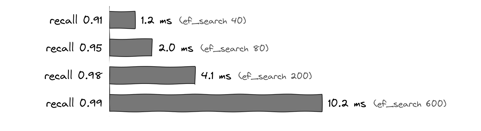
Figure 1. Median latency of one pgvector HNSW query. pgvector 0.8.7, m = 16, ef_construction = 256, 64-vCPU server, one client, a single 10-second run per point. Figure from the talk slides.
Sending one query at a time to the same index, the median latency was about 1.2 ms at recall 0.91 and about 10.2 ms at recall 0.99, roughly 8x. Going from about 0.98 to about 0.99 added about 6.1 ms, while the whole latency at about 0.98 was about 4.1 ms. The last point of recall cost more than everything before it.
So a throughput or latency figure without its recall cannot be read: giving up a little accuracy can always buy speed. In the talk we compared only at similar accuracy, and the main result was measured at a recall of 0.99 or higher on both sides. The index in Figure 1 (ef_construction = 256) is a different build from the one in the main result (ef_construction = 200).
Build time against query throughput, at the same recall
An HNSW index has two build settings. m is the maximum number of connections per layer of the graph, and ef_construction is the size of the candidate list during the build. Raising either makes the build slower. The table shows four pgvector indexes on the same data, each tuned to a recall of 0.99 or higher.
m / ef_construction | Build time | ef_search to reach 0.99 | Throughput (16 sessions) |
|---|---|---|---|
| 16 / 128 | 54 s | 1000 | 866 QPS |
| 16 / 200 (used for the talk's main result) | 67 s | 640 | 1,210 QPS |
| 16 / 400 | 109 s | 480 | 1,470 QPS |
| 32 / 400 | 157 s | 240 | 1,686 QPS |
64-vCPU server (m8id.16xlarge), 63 parallel build workers, means of five builds per setting. Throughput is 9,000 evaluation queries over 16 sessions divided by their time, not the pgbench measurement used later in this post.
Among the four settings in this table, the more time an index spent in its build, the smaller the ef_search it needed to reach recall 0.99, and the faster its queries were. The cheapest build, 16/128, reached 0.99 only with ef_search at pgvector's limit of 1000, and it had the lowest throughput. For these four settings, at a fixed recall, build time bought query throughput. A longer build does not always mean faster queries, so this relation should not be carried over to other settings as it is. The two ends of the table differ by about 1.9x in throughput and about 2.9x in build time. Fixing the recall does not finish the comparison; both the build settings and the search setting have to be written down for anyone to get the same number again.
Two cautions. First, building the same setting five times moved recall near 0.99 by 0.3 to 0.7 points. The ef_search values in the table are where the five-build mean crosses 0.99, so a single build could have led to a different choice. Second, only 16/200 was measured repeatedly with pgbench across client counts up to its peak throughput. The faster settings in the table were not measured that way. A single-run sweep of other settings is reported below, in the section on comparing best against best.
The same problem appears when comparing build times. On one million vectors, the whole CREATE INDEX took about 67 s for pgvector 16/200, about 31 s for CAGRA, and about 27 s for the GPU-built HNSW (ef_construction = 128), each a median of five runs. But the cheapest pgvector build that reaches recall 0.99 is 16/128 at 54 s (a mean of five builds). Against 67 s, the GPU-built HNSW is about 2.5x faster to build; against 54 s, the ratio is smaller. That is why the talk gave ranges: about 27 to 31 s on the GPU, 54 to 67 s on 64 vCPUs. The two HNSW builds also used different ef_construction values, 200 and 128, and that belongs next to the number.
Read throughput together with latency
We applied concurrent load with pgbench in a closed loop: each client sends its next query as soon as it gets an answer. We raised the client count from one, measured each count for 60 seconds, five times, and took the median. The GPU side was a 24-vCPU server with one A100; pgvector ran on a separate 64-vCPU server. The full conditions and the results table are in the earlier post.
What we learned here is that a peak throughput says little without the client count that produced it and its latency. pgvector peaked at about 3,550 QPS with 64 clients, at a p99 of about 27 ms. CAGRA with a 200 µs batching window peaked at about 6,520 QPS with 32 clients, at a p99 of about 7.7 ms. The two p99 values come from different client counts. Past its peak, throughput fell: pgvector delivered about 3,130 QPS at 128 clients. Finding a peak means pushing the client count beyond it.
Starting from a latency budget changes the comparison. With a p99 budget of 10 ms, every point of CAGRA with the window from 1 to 32 clients was inside it. pgvector, at the setting we measured (16/200, ef_search = 640), had no point inside it; its lowest p99 was about 17 ms, with one client. "About 1.8x the throughput" and "no point inside the budget" come from the same measurement but answer different questions. A faster pgvector setting might change that latency. In the single-run sweep reported in the next section, the fastest setting at recall 0.99 or higher had a p99 of about 11 ms with one client.
The load you measure under also decides which setting looks good. The batching window raised throughput about 4x with many clients, but with one client there was nothing to wait for, so it only added delay: one-client throughput dropped from about 1,180 to about 890 QPS. Measured under only one of those loads, the window would have been judged the opposite way.
Systems with different settings are compared best against best
pgvector's HNSW and CAGRA cannot be given the same settings and then measured. The build settings are m and ef_construction on one side and graph_degree and intermediate_graph_degree on the other. The search setting is hnsw.ef_search on one side, and cuvs.itopk_size and cuvs.search_width on the other. The hardware cannot be made equal either: one runs on CPU cores, the other on a single GPU. The only thing both sides can be set to equally is the outcome, recall. The comparison of direct calls with the PostgreSQL path, covered later, runs the same CAGRA index through two paths, so its points can be paired by setting. Between two different products there is no such pairing.
So the basis of the comparison is not "the same settings" but "each side's best at the same recall". For that comparison to be fair, the tuning points that decide each product's performance have to be examined thoroughly. The ones we varied here were m, ef_construction and hnsw.ef_search for pgvector, and graph_degree, intermediate_graph_degree, cuvs.itopk_size, cuvs.search_width and the batching window (off and 200 µs) for CAGRA. In the talk's main result, the only search-side setting we fixed for CAGRA was the candidate count, cuvs.k, at 100. If one side runs at a well-tuned setting and the other at a poorly tuned one, the gap measures the tuning, not the two systems. The settings table above shows how large that can be. Within pgvector alone, throughput at recall 0.99 or higher differed by about 1.9x depending on the settings. In the talk's main result, the peak throughput of the two systems differed by about 1.8x. The two figures were measured differently and cannot be set directly against each other, but they do show that the choice of the other side's setting can make a difference as large as the one in the conclusion.
Best also covers the environment, not only the settings. We ran pgvector on a separate 64-vCPU server rather than on the GPU server's own 24 vCPUs, and checked on every build that 63 parallel workers had attached. On the CAGRA side we turned on the 200 µs batching window, which groups queries from many clients. The window is off by default, and as the earlier post reports, peak throughput without it was about 1,560 QPS.
Time, hardware or other constraints can make it impossible to examine the tuning points thoroughly. When that happens, what was left unexamined must be stated alongside the result. Each of our own two measurements meets only half of this standard. The main result gave each side a suitable environment but used one setting per side. Figure 2 in the next section does the opposite: it sweeps the settings on both sides and takes each side's highest throughput at each recall, but pgvector ran on the GPU server's 24 vCPUs.
The 16/200 setting used for pgvector in the main result is not its fastest on that server. Two days before the talk we started a separate 64-vCPU server of the same instance type and swept 150 pgvector settings (15 builds, 10 ef_search values), once each. At recall 0.99 or higher, the fastest point was m 36, ef_construction 256, ef_search 200 (recall about 0.991): about 6,080 QPS with 64 clients, at a p99 of about 18 ms. On the same server, 16/200 (ef_search 640), measured once for 60 seconds under the main result's conditions, gave about 3,900 QPS, about 10% above the 3,550 QPS of the main result. That sweep used one build and a single 10-second run per point, with only 1 and 64 clients, so it cannot be set directly against the main result, which is five runs of 60 seconds. We ran out of time to measure that setting again the way the main result was measured, and the talk reported the 16/200 figures. So the 1.8x is not a figure against pgvector's best, and we expect the throughput gap against a better-tuned pgvector to be smaller than that. A measurement with both sides at their best, repeated the same way, does not exist yet.
Each side's best cannot be found by picking one setting by hand. The settings have to be swept, and the next section covers how.
A whole curve instead of one threshold
The talk's main result compares one setting on each side: ef_search = 640 for pgvector and cuvs.k = 100 for CAGRA, with each index's search setting picked on calibration queries before the run. That kind of comparison is an operating point. It answers "how did these two settings do at recall 0.99 or higher", and nothing about what happens if you relax recall a little.
To answer that, you sweep the settings and draw a Pareto curve. Measure every combination of build and search settings, plot each as a point, and keep only the points that no other point beats, meaning no other point has both higher recall and higher throughput (or lower latency). Joined up, the kept points show the best each index can do at each recall.
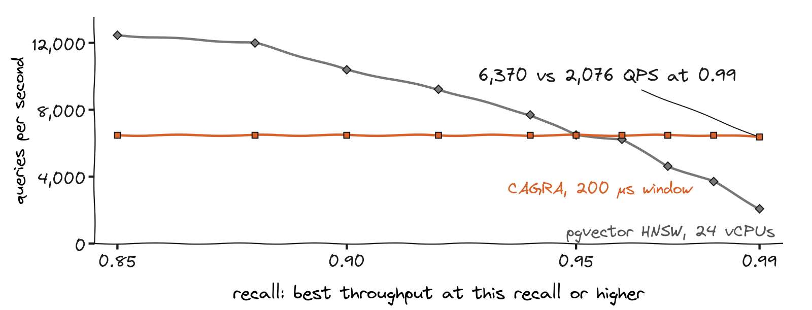
Figure 2. Best throughput at each recall or higher. Same A100 server, pgvector on that server's own 24 vCPUs, 64 clients, one run of the whole grid (315 CAGRA settings, 150 pgvector settings). Figure from the talk slides.
Each point in Figure 2 is the highest throughput among settings at that recall or higher. At 0.99 or higher, CAGRA with the window served about 6,370 QPS and pgvector about 2,080, about 3.1x. At 0.95 or higher, it was about 6,470 against about 6,490, nearly equal. At 0.90 or higher, pgvector served about 10,390 QPS, about 1.6x CAGRA, and at 0.85 or higher about 12,450. CAGRA's curve was almost flat: its best point at 0.85 or higher was the same point as its best at 0.95 or higher.
A comparison at 0.99 and a comparison at 0.90 reach opposite conclusions, and both are correct measurements. The whole curve shows which side leads in which range; a single-threshold comparison picks one point on it. This figure is what let the talk say that the GPU leads where very high accuracy is needed.
The comparison has limits. pgvector in Figure 2 ran on the GPU server's own 24 vCPUs, not the 64-vCPU server of the main result. At recall 0.99, the main result was about 1.8x and Figure 2 about 3.1x, but the two differ in CPU server and in run, and one is a single setting while the other is the best point on a curve, so the difference cannot be put down to any one cause. The only sweep of pgvector settings on a 64-vCPU server is the single run reported in the previous section. Of that sweep, only Figure 1 (one build, one client) appeared in the talk; the 64-client results did not. Where the two curves would cross with pgvector on that server cannot be read from this figure. Figure 2 is also a single run of the grid.
Compare two curves through matched pairs
With two Pareto curves on one chart, it is easy to read the gap between them as the difference between the two paths. We had to watch for this when measuring what the path through PostgreSQL costs. The question: for the same CAGRA setting, how much slower is one query through PostgreSQL and the pg_cuvs daemon than a direct call to cuVS? We ran the CAGRA grid of cuVS Bench, the benchmark tool in the cuVS repository, both ways on the same A100 server.
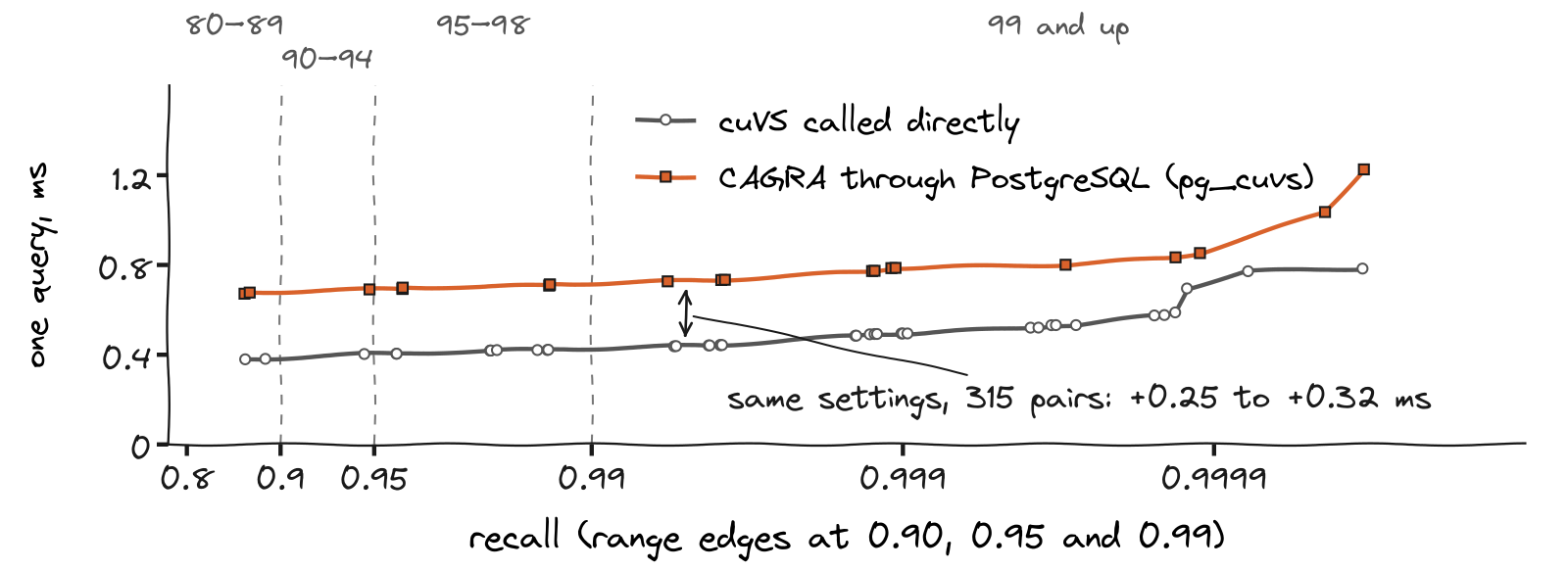
Figure 3. Pareto curves for direct calls (grey) and through PostgreSQL (orange). Same A100 server (24 vCPUs), 1M x 768, 9,000 evaluation queries, single runs. The horizontal axis spreads recall out as it approaches 1. Figure from the talk slides.
Each curve in Figure 3 is that path's own Pareto line. At the same recall, the point on the grey curve and the point on the orange curve are usually different settings. The right-hand ends of the two curves, for example, come from a build with graph_degree 64 on the direct side and 96 on the PostgreSQL side, and that is where the curves pull apart. So the gap between the curves does not answer "how much slower is the same setting through PostgreSQL".
That answer comes from matched pairs. In all 315 pairs, nine builds times 35 search settings, the path through PostgreSQL added 0.25 to 0.32 ms per query (median about 0.29 ms). While the direct latency rose along its curve from about 0.38 ms to 0.78 ms, the added cost stayed within that range. Each of the nine builds also took about 15 s longer (14.96 to 15.86 s); the earlier post covers where those seconds went.
The conditions belong with the result. The direct side is cuVS Bench 26.04 with one thread and batch size 1, reporting mean latency. The PostgreSQL side is pg_cuvs 0.9.2 with one pgbench client and no batching window, reporting the median (p50). The statistics differ: mean on one side, median on the other. The PostgreSQL side ran once, 10 s per point, and the two paths used different libcuvs builds (public and patched). The recall ranges on top of the chart (80-89, 90-94, 95-98, 99 and up) mark which points have similar accuracy.
Two mistakes in our setup
We made two mistakes in our own benchmark setup, and each changed the picture. In the talk they were on a slide that I skipped for time. Both came from runs before the formal measurement, on the same 64-vCPU server.
The first: pgvector's parallel index build ran with 6 workers instead of 63. The one-million-vector build took 180 s, and the GPU-built HNSW (25 s) looked about 7.2x faster. After the fix, under the same run conditions, the pgvector build took about 67 s and the ratio was about 2.6x. That 67 s is a different measurement from the formal 67 s above. The fix changed max_worker_processes and the table's parallel_workers together, so we could not tell which of the two had held the worker count down.
The second: we gave hnsw.ef_search a value above pgvector's limit. In the pgvector 0.8.7 source, the valid range is 1 to 1000 and the default is 40. The run with the out-of-range value ran at the default of 40, and its one-client throughput of 867 QPS was a number at recall 0.90. The formal measurement on the same server, tuned to recall 0.99 or higher (ef_search = 640), gave 87 QPS, about a tenth.
The two mistakes pushed in opposite directions. The first made the GPU look better than it was; the second made pgvector look faster than it was. Afterwards we changed how we measure:
- Count the parallel workers that actually started, for every build.
- Record recall with every number. Written next to recall 0.90, the 867 QPS of the second mistake shows up as a number outside the target.
- Use separate queries for choosing a search setting and for measuring the result.
- Run pgvector, the comparison partner, on a separate 64-vCPU server rather than on the CPU that comes with the GPU server, and repeat five times.
Limits of this comparison
- One dataset (1M x 768), one GPU type (A100 80GB), two index types. Nothing here shows that other data or other indexes behave the same way.
- The main result compares one setting per side. Figure 2, which covers the whole recall range, comes from a different CPU server (24 vCPUs) and a single run. The sweep of pgvector settings on a 64-vCPU server is one run of 10 seconds per point, and a measurement with both sides at their best, repeated the same way, does not exist yet.
- Throughput in the settings table is an approximation, not pgbench.
- The direct-versus-PostgreSQL pairs are single runs, with different statistics (mean and median) and different libcuvs builds on the two sides.
- We did not compare cost in money.
- All measurements were made inside the project and have not been reproduced elsewhere.
The pg_cuvs code is at pg-cuvs/pg_cuvs[2].
References · 2
- [1] PGConf.Asia session page — pgconf.asia
- [2] pg-cuvs/pg_cuvs — github.com