What Happens to HNSW Recall After Adding Vectors? (1M+1M)
A 1M+1M insertion study in pgvector and Qdrant, comparing insertion order, batch boundaries, and fresh indexes. Segment telemetry and version-pinned code help explain their different behavior.
In an earlier experiment, we added 10,000 vectors to an index of 10,000. The recall differences between insertion paths and freshly built indexes were small. This follow-up asks the same questions at 1 million existing vectors plus 1 million incoming vectors.
The direction of the before-and-after change differed between products. Recall@100 fell in pgvector and rose in Qdrant, including when both used the same construction parameters. Looking at the execution records revealed another change: Qdrant searched a different number of HNSW graphs before and after insertion.
This post follows the evidence from insertion paths to the storage and search structures behind them.
Compare the data states before explaining the change
We used public MS MARCO SimANS embeddings: 768-dimensional float32 vectors, searched by their original inner product. Each product started with one million vectors. We added the same incoming million through four paths and built a separate fresh index from the final two-million-vector set. The fresh control was a separate load and build, rather than an in-place reindex of an incremental index.
| Item | Configuration |
|---|---|
| Versions | PostgreSQL 17 / pgvector 0.8.7; Qdrant 1.17.1 |
| Construction | Both products: M=16, ef_construction=100 |
| Search ef | All of 100, 128, 256, 512, 1000 |
| Evaluation | Input seed 11; the same 200 queries |
| Build repetitions | One per condition |
| Ground truth | Exact top-100 over the vectors present at each checkpoint |
The products ran separately on the same CPU VM class. The following example uses search ef=256 and Recall@100.
| State | pgvector | Qdrant |
|---|---|---|
| Initial 1M | 76.880% | 81.705% |
| Final 2M after random-order insertion | 74.685% | 83.745% |
| Fresh final 2M | 74.655% | 83.155% |
| Final incremental minus initial | −2.195 pp | +2.040 pp |
| Final incremental minus fresh | +0.030 pp | +0.590 pp |
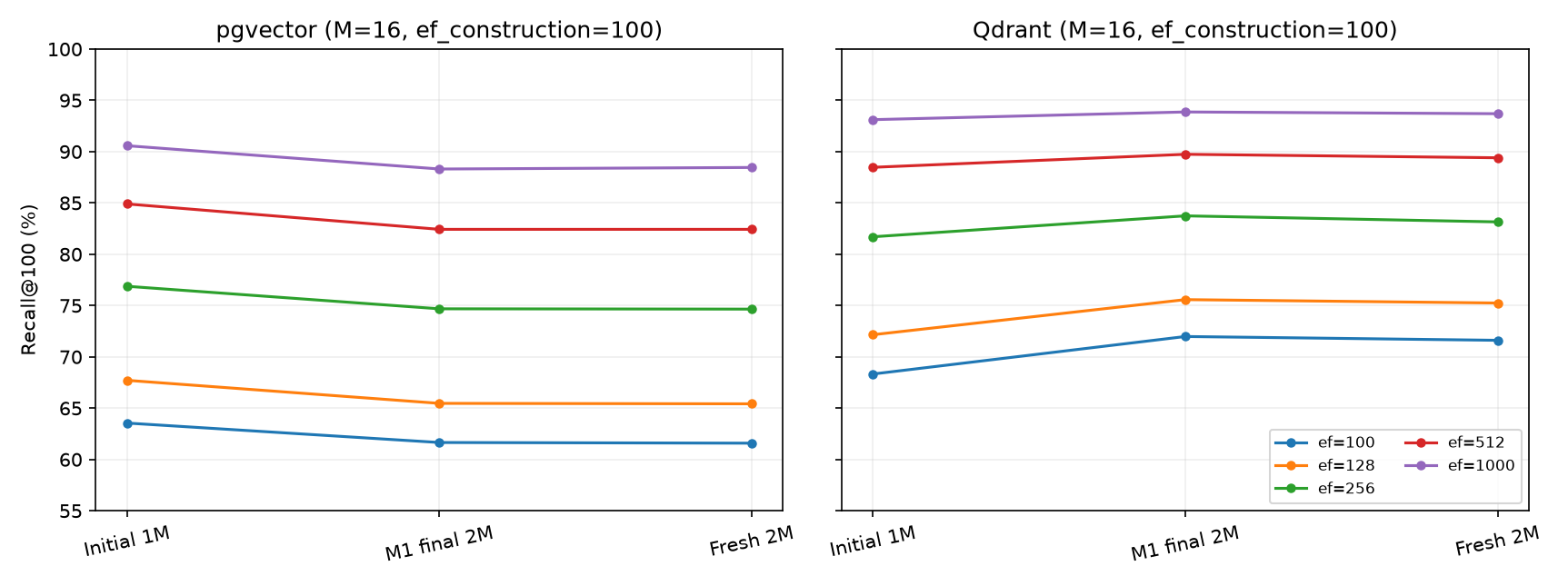
Both products show all five ef values. Each line color identifies one search ef.
The pgvector index lost 2.195 percentage points relative to its initial state, but differed from the same-final-data fresh index by just 0.030 points. Qdrant gained 2.040 points over its initial state and exceeded fresh by 0.590 points.
These are different comparisons. Adding data changes the true neighbors as well as the index. Across four final insertion paths and five ef values, incremental-minus-fresh Recall@100 ranged from −0.730 to +0.480 pp in pgvector and −0.755 to +0.670 pp in Qdrant.
Order and batch boundaries
We created a random permutation of the incoming million vectors and a clustered order using five spherical k-means clusters. Clustering used normalized copies; the databases received the original vectors.
| Path | Order | Logical waves |
|---|---|---|
| M1 | Random permutation | 1 |
| M5 | The same permutation as M1 | 5 |
| C1 | Grouped by cluster | 1 |
| C5 | The same clustered order as C1 | 5 |
The five wave sizes were 353,849 / 124,116 / 254,129 / 173,389 / 94,517. M5 used the same sizes as C5. Each product restored the same initial physical index snapshot for its four paths.
Transport batches were 1,000 vectors in every path. A five-wave run paused for indexing readiness, verification, and search between waves.
At ef=256, the final Recall@100 differences were:
| Comparison | pgvector | Qdrant |
|---|---|---|
| Random: five waves minus one, M5−M1 | +0.450 pp | +0.080 pp |
| Clustered: five waves minus one, C5−C1 | +0.005 pp | +0.160 pp |
| One wave: clustered minus random, C1−M1 | +0.150 pp | −0.830 pp |
| Five waves: clustered minus random, C5−M5 | −0.295 pp | −0.750 pp |
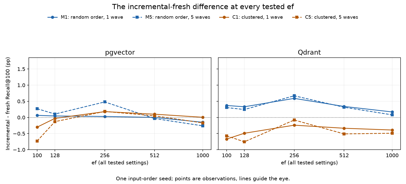
Blue is random order and brown is clustered order. Solid lines are one wave; dashed lines are five waves. The vertical axis is the difference in percentage points.
Qdrant's clustered order had lower Recall@100 than the random order at the same wave count across all five tested ef values. In pgvector, the sign of the order difference depended on ef. Splitting was also mixed: Qdrant's M5−M1 was positive only at ef=256.
One graph across pages, or one graph per segment
A pgvector HNSW index spans PostgreSQL pages. Neighbor references connect nodes across those pages, forming one logical graph. Online insertion searches that graph and updates neighbor connections. pgvector structures[1], insertion implementation[2]
A Qdrant segment holds vectors, IDs, payloads, and indexes. Search can traverse an independent HNSW graph in each segment and merge its candidates with the others. New vectors enter appendable segments, while the background optimizer schedules indexing and merges. Qdrant segment search[3], indexing optimizer[4]
The five input clusters were an experimental choice. They did not correspond to five Qdrant segments.
The telemetry showed two graphs becoming three
We inspected the completed Qdrant M1 run at ef=256.
| State | Nonempty HNSW segments | Vectors per segment | HNSW counter increase over 200 queries |
|---|---|---|---|
| Initial 1M | 2 | 683,000 / 317,000 | 400 |
| Incremental final 2M | 3 | 683,000 / 683,000 / 634,000 | 600 |
| Fresh final 2M | 3 | 683,000 / 683,000 / 634,000 | 600 |
Each state also contained one empty segment. Every nonempty segment's HNSW search counter increased by 200. Plain and exact search counter increases were zero. One initial segment UUID remained at the final checkpoint; the other was replaced by new segment UUIDs.
So ef=256 described a different search structure before and after insertion: two independently searched graphs initially, and three at the end.
This is a plausible contributor to Qdrant's rising recall. More independent segment-local searches provide different opportunities to discover candidates. But ef is not a count of visited nodes: three searches at ef=256 do not mean exactly 768 node visits or three times the computation.
The M1 and fresh final indexes also searched three graphs each, yet differed by 0.590 percentage points. Segment count alone does not explain that difference. Their vector membership and graph connections still matter.
Candidate merging need not lose the global answer
If every segment returns its exact top-100, merging those candidates and selecting the best 100 recovers the global exact top-100. A vector outside its own segment's top-100 already has at least 100 better vectors ahead of it, so it cannot enter the global top-100.
With ANN, the graph search may fail to produce the right candidates. That is where approximation enters this comparison. This Qdrant run searched all nonempty segments rather than routing each query to only a selected subset.
The lifecycle resembles ClickHouse MergeTree parts: create or fill separate units, consolidate them in the background, and combine their query results. MergeTree parts are immutable, whereas Qdrant also has appendable segments. For ordinary exact MergeTree queries, reorganizing the same data preserves the answer. With HNSW, changing graph membership and the number of searches can also change recall at a fixed ef. ClickHouse part structure[5]
Why did clustered order behave differently in the two products?
Clustered order hurt Qdrant at all five ef values. pgvector showed no such consistent disadvantage. The architectural question is how input order leaves a trace in the final index.
For each new vector, pgvector searches the existing HNSW for neighbors and links the node into that graph. It also updates existing nodes' neighbor lists, selecting neighbors again when a list reaches its limit. The code follows HnswFindElementNeighbors → UpdateGraphOnDisk. Even when cluster B arrives after cluster A, B searches the shared graph containing the initial million vectors and earlier insertions. pgvector insertion code[2], Neighbor updates[6]
If the initial graph already connected the regions occupied by the incoming clusters, those connections could have softened the effect of their arrival order. Splitting insertion into five waves also continues updating that same graph. HNSW construction remains order-dependent in pgvector, but this run showed no consistent recall penalty for clustered order.
In Qdrant, arrival order can also affect which vectors share a segment. Random and clustered arrivals can leave different vector distributions in a segment when an optimizer runs. Each HNSW selects neighbors from its own segment's vectors. Waiting for optimization between waves can change which data is indexed or merged together. Construction includes paths for reusing and healing an existing graph, as well as parallel insertion. Segment optimization code[7], HNSW construction code[8]
The final M1 and C1 states both had three graphs containing 683,000 / 683,000 / 634,000 vectors respectively, yet C1's Recall@100 was 0.830 points lower at ef=256. Graph count alone cannot explain this order difference. Different segment membership and the connections formed within each graph offer a possible explanation. Every nonempty segment was searched; the relevant issue is how well each graph found its true-neighbor candidates.
This is an architectural mechanism through which order can affect Qdrant. Grouping similar vectors can also make a graph easier to search, however. We have not compared segment membership and graph connections closely enough to establish why clustered order hurt in this run.
Average differences and per-query outcomes
We recomputed per-query Recall@100 from Qdrant's raw returned IDs and the shared exact truth. These counts compare the left path with the right at ef=256.
| Comparison | Mean difference | Lower recall | Tied recall | Higher recall |
|---|---|---|---|---|
| C1−M1 | −0.830 pp | 108 | 29 | 63 |
| C5−M5 | −0.750 pp | 105 | 27 | 68 |
| M5−M1 | +0.080 pp | 80 | 38 | 82 |
M5 and M1 differed by only 0.080 points on average, but 162 of the 200 queries had different recall. Clustered order lost on more queries than it gained, while still improving some queries. A small average gap contained different outcomes for individual queries.
Qdrant also lost with clustered order at the higher construction setting
Was Qdrant's disadvantage for clustered order specific to M=16 and ef_construct=100? The earlier M=48, ef_construct=300 run showed the same relationship: at the same number of waves, clustered order had lower recall than random order. This held at all five search ef values in both construction configurations.
The differences at ef=256 show which relationships persisted and which changed. Values are Recall@100 percentage points.
| Comparison | M=16, ef_construct=100 | M=48, ef_construct=300 |
|---|---|---|
| Clustered minus random, one wave: C1−M1 | −0.830 | −0.215 |
| Clustered minus random, five waves: C5−M5 | −0.750 | −0.335 |
| Five minus one wave, random: M5−M1 | +0.080 | −0.725 |
| Five minus one wave, clustered: C5−C1 | +0.160 | −0.845 |
At this ef, the clustered-order disadvantage was smaller at the higher setting, but remained present. Splitting behaved differently. At the higher setting, five waves lost to one wave for both input orders, and did so at all five ef values. C5 had the lowest recall of the four insertion paths throughout that sweep.
The reference matters here. At the higher setting, C1 beat fresh by 0.675 points but lost to random-order M1 by 0.215 points. Beating fresh did not make clustered order better than random order. A fresh build and the different insertion paths produced different results over the same final vectors.
Did a fresh build give better recall?
In this 1M+1M experiment, indexes that received new vectors did not consistently fall below fresh. With M=16 and ef_construction=100 in both products, every incremental-minus-fresh gap was within one percentage point, with both positive and negative results. For pgvector, random insertion in one wave differed from fresh by 0.030 points at ef=256. For Qdrant, random insertion beat fresh at all five ef values. Building anew over the final two million vectors did not consistently raise recall in this comparison.
Insertion did change recall. Random insertion in one wave lowered pgvector's recall by 2.195 points from its initial value, yet fresh ended up at almost the same level. Treating that entire before-and-after drop as damage to the existing graph would also count changes arising as the dataset doubled.
Qdrant moved in the opposite direction: recall rose after insertion, while the number of independently searched HNSW graphs grew from two to three. pgvector added nodes to one connected graph; Qdrant changed its segment layout and gathered candidates from several graphs. Keeping ef fixed therefore did not keep the search structure fixed. This provides one explanation for the different directions of the products' before-and-after results.
Insertion method still mattered. In Qdrant, clustered order lost to random order at both construction settings. pgvector showed no consistent disadvantage for clustered order. Splitting offered no shared advantage either; at Qdrant's higher setting, it hurt both input orders. Adding vectors did not automatically degrade these indexes, but the same incoming vectors could still produce different final recall depending on their order and how insertion was split.
References · 8
- [1] pgvector structures — github.com
- [2] insertion implementation — github.com
- [3] Qdrant segment search — github.com
- [4] indexing optimizer — github.com
- [5] ClickHouse part structure — clickhouse.com
- [6] Neighbor updates — github.com
- [7] Segment optimization code — github.com
- [8] HNSW construction code — github.com